Chapter 2 Place in transit data

Words like place, location, and position are commonly used in transit planning and transit data modelling. Just like time, these words are overloaded. I have noted that it’s often not that clear what exactly is meant: instead, it must be figured out implicitly from the context, which is not always easy, especially for new people, such as software developers, who are only underway onboarding the business domain. We could do better documenting our assumptions and mental models of these terms and their usage.

In this text, I’ll try to open up my thoughts about the meanings of place, location, and position when it comes to transit vehicles. There’s of course much more to the topic than this - for instance, meanings of place for passengers moving in the transit system would be a whole different story, but I’ll not go into that this time.

About the three terms: I know there are different personal connotations, as well as more or less different official meanings, to place, location, and position. Unfortunately at HSL, at least, we don’t have exhaustive definitions for these words to use in data models, for instance, and I think in practice we have a lot of overlap in their usage. I’ll not try to give the right answer to the definition question in this post. Rather, I’ll be using any one of these for approximately same meanings. Perhaps one nuance to note is that I consider place a more general, area-like term, while location and especially position refer to a more or less exact point in a space. You may well agree or disagree with me!

2.1 Stops - anchor points for vehicles (and passengers)

I’ll first discuss transit stops, because they are such an essential part in defining where a vehicle is located in a transit system.

A stop is a basic unit in a transit system in many ways. It is the service interface for passengers who use stops to enter and exit transit vehicles, to wait for them, and to transfer between vehicles. Conversely, for the transit vehicles, stops are usually the only allowed areas to open and close doors, and serve passengers. Therefore, stops comprise the important network of places that any transit system is based on. Strictly thought, the space in between stops is not accessible to passengers (as long as they are travelling by transit and not by walking, for instance).

Stops can be grouped together into more general constructs: most often, stations and terminals are technically collections of stops. GTFS specification uses the parent_station attribute to enable this, for example. It may be relevant as well to add grouping labels to stops on opposite sides of a road: technically, such stops are totally separate points of service, they almost never even serve the same route/direction variants, but from a passenger’s point of view, they are considered very much belonging to the “same area”. The same applies even more to multiple stops on different sides of an intersection, which are often used for transfers.

In schedule run time planning, described in more detail in Chapter 1, not all stops belonging to a route or to a section shared by more routes are relevant, not even nearly. As long as there are several successive stops on a route in a similar traffic infrastructure and having similar passenger demand patterns, the real stop-to-stop vehicle run times tend to behave in a quite linear manner, i.e., the mean speed remains almost constant over multiple stop intervals. Thus, we need to define separate run times only when the mean speed and the conditions defining it change significantly, or whenever we want to define a holding regime (regulating stop) to a stop, to prevent vehicles from departing early. The schedule planning software used at HSL, HASTUS by GIRO Inc., uses the term stop place to label stops for these purposes.

In practice at HSL, certain stops get place labels upon need as global attributes, and to actually use a stop as a scheduling or regulating place on a route, the place needs to be activated for that route (+ direction and variant). This is because stops may have different roles in different routes, for instance due to different usage patterns by passengers, or because a stop is used for regulating on route A but not on route B. Even more importantly, places are yet another way to group together multiple stops, and often this means even adjacent stops in the same direction on the network; to use places reasonably on a route, only one stop of each place must be chosen for each route.

2.1.1 Are stops points, areas, or linear features?

Stops are most often understood and modelled as points, which makes a lot of sense. Usually the point on a map shows where the stop pole, and possibly shelter, is located, and this point is then easy to navigate to and from, both to passengers and vehicle drivers. Thus I’d say that a point geometry is a bare minimum a stop must have in a transit data model, in addition to a unique stop id.

In reality however, we see that stops require some area to work - vehicles cannot stop and passengers cannot wait at a singular geographical point. Practically, vehicles serving passengers always reserve a certain length of the street, or possibly a stop pocket on the side. To match these vehicles to the stop point they are currently serving, we need to model this pocket, or a piece of street, in our data model. Some error margin should also be included, to address random jitter that is inherently there with vehicle GPS signal. An answer to this is stop radius that defines a reasonable area, 20 or 30 meters for example, around the stop point geometry. The resulting circle is then used to match any vehicles inside it to the stop. The circle alone is not enough, though: to not match vehicles that happen to traverse through a stop they are not meant to serve according to the scheduled route, the list of route stops (stop pattern) must be involved in the matching algorithm.

A common problem with stop circles is that since they have to be defined large enough to catch some outliers too, due to GPS jitter, they might grow so large that they start catching vehicle GPS position that they should not. For instance, a route geometry may often do a “stitch” - visit a dead-end street and then traverse it back to another direction - and such a case often results in vehicle-to-stop matching done too early or late. Another source of error are zigzag-like, self-intersecting route geometries in terminal areas where the same stop radius may again be traversed multiple times by the route, and at the same time, especially in inside terminals the stop radius may be extremely large due to unusually large GPS jitter.

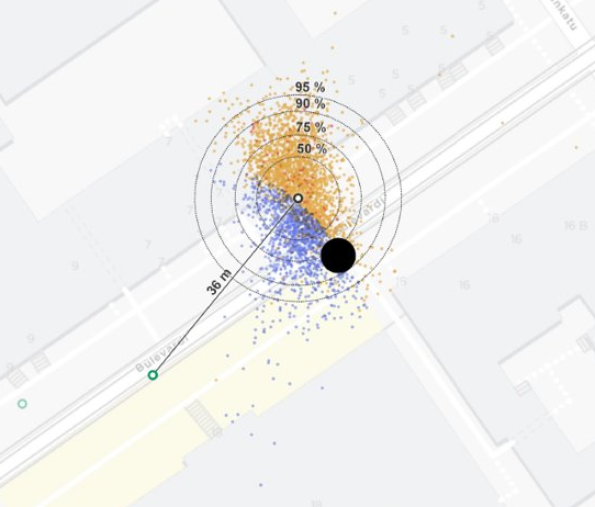
Figure 2.1: Example of mismatch between modelled and actual stopping locations in Fredrikinkatu, Helsinki.

Figure 2.1 shows an example of a tram stop in Fredrikinkatu/Bulevardi streets in Helsinki, where we have a tram stop modelled in the pole position, but the actual GPS locations of stopped trams (here, from one week) are significantly offset from that point. Blue dots have had the correct stop_id matched, while the others didn’t have the stop recognized. We can clearly see where the stop radius goes, 35 m around the stop point in this case. The example area has significant GPS jitter probably due to high houses and a narrow street.

To address the aforementioned accuracy problems, stops could be modelled as arbitrary polygons that reflect the real areas actually taken by vehicles - or at least, how GPS sees that area. While this requires some human effort, it could reduce the amount of matching errors. Another alternative could be to always match vehicle positions to the street link they are currently using, and mark the stop coverage area as a length interval on the link, or on several successive links. It would then be the responsibility of the GPS-to-street matching algorithm to handle outliers correctly - include or leave them out depending on the route geometry that the vehicle should be following, for example - and the remaining matched points on the links would be a pretty reliable source for stop matching.

A downside of these more precise methods, arbitrary polygons or linear distance coverage intervals, is that they are harder to calculate in realtime environments, and probably harder to debug as well. A stop radius provides a really straightforward basis for calculations in 2D coordinates - it’s just about whether the Euclidean distance between the stop and vehicle position falls under a given limit.

Ideally, all of these methods could be used in a data model, each fitting best a certain purpose: stop pole/shelter point would work for passenger information, there might even be another point representation for median stopping location, then a radius around it to use quickly in realtime matching, and finally, a polygon and / or a linear distance coverage interval to use for more precise and reliable data processing afterwards, when calculating KPIs based on realized stop arrival and departure times, for example.

• Be consistent and careful in how you determine the point location of a stop in your data model. Is it to always represent where the stop sign pole is located? Or does it rather represent the median or average position where vehicles actually seem to stop? These can differ even tens of meters for large, busy stops.
• For the aforementioned reason, do not rely on modelling your stops as points only. At least a radius around the point is needed to catch the vehicles that stop near the point at variable positions.
• A stop radius is straightforward to use in vehicle-to-stop matching algorithms, especially in realtime applications. However, it can be too rough for an estimate of the real area used by vehicles at that stop, especially if route geometries traverse through the resulting circle in complicated ways (common in terminal areas, especially), or if successive stops on a route end up with intersecting circles.
• To address that problem, you can model the stop area with a polygon that represents the real stopping area while leaving out “outliers”, or by defining the stop as a distance coverage interval along the related road or track links, which then catches correct distance values of vehicle positions projected to the links from GPS coordinates. See Part 2.3 for more information.

2.1.2 When is a vehicle at stop?

Stop events are realtime or historical data about actual departure and arrival times of trips by stop on a realized transit trip. They can have other stop-related attributes as well, such as door opening and closing times, and number of boarding and alighting passengers. An ordered list of stop events forms the spatiotemporal position history of a transit vehicle at the accuracy of stops. This is typically an essential source for not only transit planning processes such as run time planning, but also for various key performance indicators (KPI). In my experience, stop events are the most common type of data about realized transit operations in research papers, too.

While stop events are perhaps the most crucial type of realtime data for passenger information and history data for transit analysis, KPIs, and planning, I’d say they are not “real” events. They are artificial in the sense that they depend completely on other, multiple underlying facts: where the stop point was located in the planning database, how the effective stop area was modeled (e.g. circle or polygon around the stop), what the role of the stop was on the trip route and if there was a risk of mismatching e.g. because the route goes through the stop area twice or more; and on the other hand, the accuracy of vehicle positioning (GPS) affects the resulting stop events, too. Since stop events are so prone to various errors reducing their temporal accuracy or even preventing the events to be triggered at all, I would not recommend recording them as the only type of data about realized transit operations. Persisting original vehicle GPS tracks, their trip status history (which scheduled trip they were signed in to at each time), as well as route geometry, network link, and stop representation from the corresponding operating days forms a more reliable basis to not only calculate the stop events but also to monitor their quality, debug, and re-calculate them upon need.

Practical examples of reflecting transit vehicle location through stops are real-time arrival predictions in Digitransit (behind the HSL Route planner, for example), StopTimeEvent message type in GTFS Realtime specification, and stop-related event types in Digitransit HFP (high-frequency positioning).

• If using plain stop events in your data model without a view to how these events were generated, treat them critically. Can you trust that the stop points and areas were created realistically so the vehicles could match the stop easily? Can you trust the accuracy of vehicle computer GPS devices so they have produced precise position values when matching the stop?
• Consider if it’s possible to generate, or at least validate, the stop events afterwards with the facts needed for stop matching: pure vehicle position (GPS) data, the original stop locations and areas (such as radius around the stop point), planned trip route geometry, and the stop as part of the route. This way you can verify whether the stop matching process has worked correctly - this can be as simple a process as checking samples of GPS data together with the stops on a map.
• Using those facts rather than stop events generated on the fly in real time, you can adjust the stop location, area, and matching parameters, and re-run the matching process afterwards, if required. Having only stop events matched in real time can be pretty unreliable, since you cannot back up and fix errors like this.
• Storing all these facts and generating stop events afterwards doesn’t mean you have to store huge amounts of data. You can define a shorter lifespan for big data, such as raw GPS points: keep them as long as you need for the matching and validation process - say, a week - and discard old data regularly from your database.
• The more critical realistically functioning stop events are for your transit KPIs, the better you should log and monitor their data quality and reliability of their generation process.

2.2 What is between stops

Transit vehicles do not jump from stop to stop, they have to find their way there through a decent path on the transport network. From passenger’s perspective, a vehicle can be “stopped at” a stop and thus available to enter and exit from, or not available: “incoming at” (just about to arrive) or “in transit to” (underway) to the next stop. This is how GTFS Realtime sees it. Meanwhile, there’s a whole lot going on to the vehicle driver: the exact itinerary to follow in the street network, and various reasons to slow down, stop, and accelerate again, whether it be due to other movers in the same space, traffic lights, or weather conditions. A transit planner or analyst should interested in these between-stops factors as well, since they all contribute to the run times between stops that we wish to minimize for fast service. At least, we want to minimize the variability - unreliability, randomness - of them.

In this regard, it is important to identify routes that vehicles follow not only in terms of ordered stops, but also in terms of an exact path of street or track link geometries in the network. Ideally, the path tells about not only the geographical characteristics but also what features and circumstances are involved: traffic lights, pedestrian crossings, bus lanes, speed limits, mean volumes of other traffic (as a proxy of mean “free” speeds in practice). And, of course, stops located along the route path. These have to be considered in two ways: firstly, stops that belong to the route and are therefore a “desired” reason for stopping, and stops as infrastructure that do not necessarily serve that very route but might cause excess stopping and waiting, e.g. due to another transit vehicle in front.

Network paths between a given pair of stops are not set in stone. Transit network are in constant change, more or less, due to infrastructure development, construction sites, temporary disruptions, and so on. For these practical reasons, actual transit vehicle itineraries need to be updated every now and then, even if the stops and their order do not change. Moreover, paths between stops are sometimes technically not the shortest paths in the first place. If they were, we could just derive the itineraries automatically from the ordered stop list, assuming we have a decent network model at hand. But this is not the case. Therefore, the stop list and network itinerary of a transit route must be maintained separately in a data model. Of course, stops and route links have common conditions that must be enforced in the data model: the stops of a route must be available at the links as well that the route uses, and those stops and links must be traversed in sync.

I wish the network aspect could be better considered in common transit data models, such as GTFS. There, changes in stop lists are pretty easy to detect between feed versions, while changes in the underlying network itineraries must be figured out implicitly from geometric differences between route shapes, or from different shape_dist_traveled values of the same pair of adjacent stops in stop_times.txt. Also in HSL Jore transit registry, network links are there under the hood, but export files and (currently almost non-existent) interfaces provide only entire route geometries and stops belonging to the route. Accessing the ordered link geometries and ids of a route would enable matching vehicles to link rather than whole route geometries, and eventually it would be easy to see which vehicles are using the same street or track link, no matter which route they are on.

• A transit route pattern can be expressed as an ordered list of stops or as an ordered list of directed street or track links. Ideally, include both of them in your data model, and make sure to validate that these two go hand in hand without logical conflicts.
• Stop and link based paths do not determine each other automatically but require human intervention. A route through a link does not necessarily use all available stops at that link. A route from stop A to stop B does not necessarily use the shortest path of links between the stops.
• Vehicle status in relation to route pattern stops, such as VehicleStopStatus in GTFS-RT, is not a fact coming out of the blue but requires a reliable algorithm to detect whether the vehicle is approaching, stopped at, or departing from a given stop. It’d be nice if your data model not only makes available not only this status information but also how it is generated - e.g., the raw GPS vehicle position, modelled stop locations and areas at that time, as well as parameters used for the matching.

2.3 Vehicles on a map or en route?

As you might have seen above, I generally assume in transit data modelling that locating a real vehicle starts from its GPS position: latitude and longitude coordinates in the WGS84 coordinate system, from which we can convert to any other system, such as metric ETRS-TM35 coordinates that are useful in Finland. This is the “purest” form of vehicle location available to us (in HSL context also publicly available in real time, through HFP), as accurate as the vehicle GPS device can provide. I recommend recording this “pure” data for analysis, KPIs, and planning purposes, not only because it enables examining vehicle movements and GPS accuracy generally in a 2D space, irrespective of the transit network (and its possible modelling errors), but also because we can then re-calculate any derivatives such as projected vehicle locations and stop events at any time from raw data, if we note any errors in the calculation parameters or reference data such as stop points or network link geometries.

By projected vehicle location I mean the linear distance value of a vehicle in relation to a network link or the whole route line geometry that the vehicle is currently traversing. This kind of data is needed for use cases like in Figure 2.2, where the route planner app needs the vehicle position not only as 2D coordinates for map rendering, but also as a numeric value that expresses its location between stops. Similarly, it can be extremely relevent for certain KPIs and transit performance analysis in general to get vehicle movements matched to corresponding line geometries, such as links, street segments between intersections, or routes, so these can be used as the common 1D dimension for analysing vehicle movements in space and time. My entire Master’s thesis project was about this matching thing.

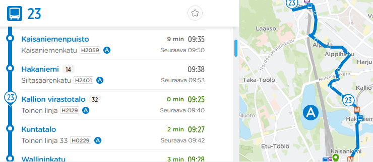
Figure 2.2: HSL Route planner showing realtime location of a vehicle along the stop list (1D, left) and on a map (2D, right).

Point-to-line linear referencing, available in PostGIS, for instance is an extremely useful tool for producing projected vehicle locations. However, only the point and line geometries are often not enough, since used alone, they can lead to incorrect matches, e.g., when a route geometry intersects itself in a loop. The matching algorithm should be able to consider other relevant facts too, such as the movement heading of vehicle position points, their speed, and a kind of a lookbehind to previous matched points to determine whether it is more realistic to match a link 5 meters away that would result in sudden jump of 250 meters forwards measured along the route itinerary, or a link 18 meters away that results in a more reasonable, 10 meters’ advance measured along the itinerary, with respect to the previous projected point. These are not always easy and intuitive to implement and debug.

2.4 Conclusion

I would say there are at least three essential ways to express where a transit vehicle serving a trip is located:

1. Plain GPS coordinates of the vehicle in 2D space.
2. In relation to road or track network: “on link X, N meters from the link start”. The distance could also be relative, i.e., a proportion from 0 to 1 of the link length.
3. In relation to stops: “at stop X” or “between stops X and Y”, possibly with a numeric value telling how much distance is left before stop Y, for instance.

Ideally, we could monitor all of these in real time, as well as store them as history data. This way, different purposes such as passenger information, transit KPIs, and planning processes based on history data, requiring vehicle position information in different formats, could all be satisfied. I think it’s important to note different needs in realtime and data warehousing contexts: in real time, all of the three ways to express the vehicle location should be available easily and quickly - in fact, the more redundancy, the better. In data warehousing on the other hand, redundancy should be avoided in my view: not only because of inefficient use of storage space and processing capacity, but also because storing these three types of data as plain results can lead to ambiguity, conflicts, and invalid data, if we note in the end that they do not fully correspond to each other. Instead, in data warehousing we should identify how each of the three data type is constructed logically from the building blocks - GPS locations, network link and stop geometries, routes as link and stop sequences - and make the three accessible as views generated by joins of these building blocks. This way, the data would remain consistent and auditable afterwards.

So, in a way, the three ways to express the vehicle location are just views to the same fact, using different frameworks: 2D map, stops, and network links.

The same logic can be applied to other essential components and actors of a transit system, too: where passengers move in time and space, and whether to inspect this “where” in relation to space, stops, vehicles, street network, and so on. Or how transit route itineraries are modelled - starting from stops or from street network links - and how stops and links are dependent on each other.

Modelling the “wheres” of a transit system requires a hierarchy of components working together from top to bottom and vice versa. Coordinate values, route geometries, stop points, and links are not enough alone, but unambiguously defined relationships between them are needed. Such a model is not easy to create, as we have seen many times in the new transit data registry project Jore 4.0 at HSL. Just try to ingest all the essentials of Transmodel as a developer without a long background in transit domain…

As with the time topic discussed in Chapter 1, I recommend not to simplify things that feel uncomfortably complex, but rather to think carefully through the complexity, and document those thoughts, mental models, related data model design decisions, and ultimately the results in understandable human language and pictures. The hardest things are not the data, code and computing themselves, but rather, getting humans to understand each other what they meant when working on these.